Machine Learning 15 Slides

Gradient Boosting The Supermodel of Machine Learning.

Slide 1 / 15

Use ← and → to navigate

Swipe left / right on mobile

Guide Notes & Explanation

Accompanying breakdown for this slide deck

Boosting is an ensemble learning technique. It combines many weak models to create one strong, accurate predictor. Think of it as a team where every member contributes a small piece to the final solution.
A weak model, often a shallow decision tree, is only slightly better than random guessing. By itself, its predictions are not very useful. The magic of boosting lies in how it strategically combines these weak links into a strong chain.
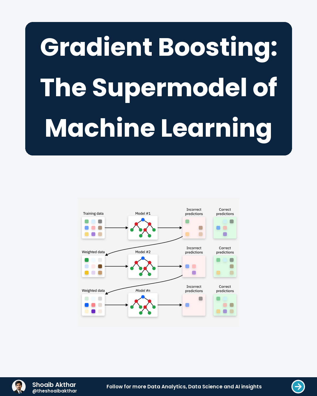
The process is sequential. Each new model is built to correct the mistakes of the previous ones. This focused, iterative improvement is the core reason for its high performance.

Gradient Boosting builds models one after the other. Each new model in the sequence focuses on the errors made by the current ensemble. The final prediction is a weighted sum of all these sequential predictions.
It is called "gradient" boosting because it uses gradient descent to minimize a loss function. The algorithm identifies the direction in which to adjust the model to reduce error most effectively. This is similar to descending a hill by always taking the steepest path down.
This method can be applied to various loss functions for regression and classification. This flexibility makes it a powerful tool for many different types of problems.

Simple models, like a single decision tree or linear regression, have inherent limitations. They often make strong assumptions about the data, like linearity, which real-world data frequently violates.
These models are prone to either underfitting or overfitting. A simple linear model might underfit complex patterns. A deep tree might overfit by memorizing the noise in the training data.
They often hit a performance ceiling. After a certain point, no amount of tuning can significantly improve their accuracy on complex tasks. Their simplicity restricts their ability to capture intricate relationships.

The process starts with an initial, naive prediction. This is often just the average value of the target variable for regression. For classification, it can be the log-odds.
This first model is very simple. It has high bias and makes significant errors. These errors, or residuals, are the difference between the true values and this first prediction.
The algorithm calculates these residuals for every data point. These residuals become the new target that the next model will try to predict.

A weak model, typically a small decision tree, is trained. But it is not trained on the original target variable. Instead, it is trained to predict the residuals from the previous step.
This new model learns the patterns in the mistakes. If the first model underestimated a group of points, this tree will learn to predict a positive residual for them. It focuses exclusively on what the ensemble got wrong.
The prediction of this tree is the predicted residual for each data point. This prediction is then used to update the overall model's output.

The prediction from the weak model is added to the ensemble's current prediction. However, it is scaled by a learning rate before being added.
The learning rate is a small value between 0 and 1. It controls how much each new tree contributes to the ensemble. A smaller learning rate requires more trees but often leads to a better model.
The update looks like this: New Prediction = Old Prediction + (Learning Rate * New Tree's Prediction). This gradual update prevents overfitting and leads to smoother convergence.

Steps 2 and 3 are repeated many times. A new weak model is built to predict the residuals of the updated ensemble. Each new model focuses on the errors that remain after all previous models have been added.
This iterative process continues for a pre-set number of rounds. The number of trees is a key hyperparameter. Alternatively, it can stop once the errors are sufficiently small.
The final model is the sum of all the initial prediction and every scaled prediction from all the sequential trees. This complex combination is what makes it so powerful.

Simple models often have high bias. They oversimplify the problem, leading to systematic errors. Gradient Boosting systematically reduces this bias through sequential correction.
Each new tree in the sequence is specifically designed to capture patterns that the current model misses. It chips away at the error from a different angle every time.
By combining many simple models, each focused on a specific type of mistake, the overall ensemble achieves remarkably low bias. It can model highly complex, non-linear relationships that a single model cannot.

Not all models in the sequence are created equal. The algorithm uses gradient descent to determine the optimal weight for each new tree's prediction.
This ensures that a tree that provides a very effective correction contributes more to the final answer. Conversely, a less useful tree has its contribution dampened by the learning rate.
This adaptive weighting is far more sophisticated than a simple average of models. It intelligently blends the strengths of each component to maximize predictive power.

Gradient Boosting is not tied to a specific type of base model, though trees are most common. This framework can work with any weak learner, providing great flexibility.
More importantly, it can use any differentiable loss function. You can customize the algorithm to minimize log loss for classification or mean squared error for regression.
This means you can tailor the model directly to the specific business problem and metric you care about. A simple model often lacks this level of customization.

XGBoost is arguably the most famous implementation. It stands for eXtreme Gradient Boosting and is known for its speed and performance.
LightGBM, developed by Microsoft, focuses on achieving similar accuracy with greatly improved training efficiency. It is designed to handle very large datasets.
CatBoost is another variant, particularly robust for handling categorical features without extensive preprocessing. All three are powerful tools that dominate machine learning competitions.

It is an excellent choice for tabular data problems where accuracy is the top priority. It regularly outperforms other algorithms on structured datasets.
Consider it for tasks like click-through rate prediction, risk assessment, and sales forecasting. Its ability to model complex interactions is invaluable for these applications.
However, it can be computationally expensive and requires careful tuning. For very large datasets or low-latency requirements, a simpler model might sometimes be more practical.

Gradient Boosting outperforms simple models by turning weakness into strength. It sequentially builds an army of simple models, each one correcting the last's errors.
It reduces bias intelligently and combines predictions optimally. This allows it to capture complex patterns in data that single models cannot see.
For any data scientist, understanding gradient boosting is essential. It is a versatile and powerful tool that provides state-of-the-art results on a wide range of challenges.