Machine Learning 15 Slides

Decision Trees — How Machines Split Decisions Like Humans.

Slide 1 / 15

Use ← and → to navigate

Swipe left / right on mobile

Guide Notes & Explanation

Accompanying breakdown for this slide deck

We make decisions every day by asking simple yes/no questions. For instance, deciding what to wear might start with "Is it raining outside?". Based on the answer, you follow a different path of reasoning.
Machines can mimic this exact same process using a structure called a decision tree. It's a model that breaks down a complex decision into a series of simpler, binary choices, just like a flowchart.
This approach is powerful because it is intuitive and mirrors human thought processes. We can easily understand and visualize the machine's "thought process" from start to finish.

In computer science, a tree is a data structure that starts with a single root node. This root represents the very first question asked or the starting point of our decision-making process.
From the root, branches extend outward, representing the possible answers to that first question. Typically, these are "Yes" or "No" pathways. Each branch leads to a new, internal node.
These internal nodes contain the next question to be asked. This process continues until a branch leads to a leaf node, which is the final decision or outcome, not another question.

The main goal in building a decision tree is to determine the best question to ask at each node. A good question effectively splits the data into two distinct groups, making subsequent decisions easier.
A perfect question would completely separate all the data points of different classes. For example, a question that puts all "cats" on one branch and all "dogs" on the other is ideal.
In reality, such perfect splits are rare. The algorithm's job is to find the question that creates the purest, or most homogenous, groups possible at every step.

To find the best split, we need a way to measure the disorder, or "impurity," within a group of data. A node is pure if it contains only one type of data point (e.g., only cats).
Several mathematical metrics exist to quantify this impurity. The three most common are Gini Impurity, Entropy, and Information Gain. Each provides a slightly different way to calculate disorder.
The algorithm will calculate the impurity before a potential split and then after. The split that reduces the impurity the most is considered the best question to ask.

Gini Impurity is a measure of how often a randomly chosen element would be incorrectly labeled if it was randomly labeled according to the distribution of labels in the subset.
Its value ranges from 0 to 0.5, where 0 indicates a perfectly pure node (all elements from one class). A higher Gini value indicates a higher level of impurity within the node.
The formula for Gini Impurity for a node is: G = 1 - sum (p_i^2) where p_i is the probability of a class i in the node.

Entropy, borrowed from information theory, measures the amount of uncertainty or surprise in a system. A pure node has no surprise and thus an entropy of zero.
A mixed node with many different classes has high entropy. The goal of a good split is to reduce the entropy, thereby increasing the certainty about the outcomes in the new nodes.
The formula for Entropy is: E = - sum (p_i * log2(p_i)) where p_i is the probability of a class i.

Information Gain (IG) is the most practical metric. It doesn't measure impurity itself but rather how much a proposed split reduces impurity.
It calculates the difference between the impurity of the parent node and the weighted average impurity of the two child nodes after the split. The weights are based on the number of samples in each child node.
The split that results in the highest Information Gain is chosen. Essentially, it identifies the question that gives us the most "information" by cleaning up our data.

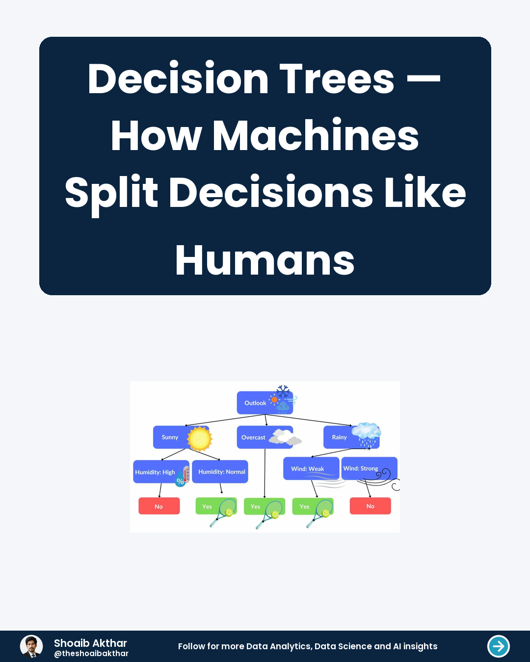
Imagine we have data on weather conditions and whether people played tennis. Our root node might contain all historical examples, both "Play" and "Don't Play".
The algorithm tests all possible first questions: "Is Outlook Sunny?", "Is Humidity High?", etc. It calculates the Information Gain for each potential split.
It finds that "Is Outlook Sunny?" creates the purest child nodes. The "Yes" branch might lead to a node where most people play, while the "No" branch leads to a new question about humidity.

The process of finding the best split and creating new nodes is recursive. It is applied to each new child node until a stopping condition is met.
These stopping conditions prevent the tree from becoming too complex. Common conditions include reaching a maximum depth, having too few samples in a node, or achieving a minimum impurity reduction.
Once a stopping condition is triggered, the node becomes a leaf node. The final prediction for that leaf is typically the most common class (mode) of the training samples that ended up there.

A deep tree with many questions can become too specific to the training data. It memorizes the noise and exceptions instead of learning the general pattern. This is called overfitting.
An overfit tree performs exceptionally well on the training data but poorly on new, unseen data. It fails to generalize because it essentially created a complex rule for every single example.
This is like memorizing the answers to a specific test instead of understanding the subject. You'll ace that test but fail any new one.

To combat overfitting, we use a technique called pruning. Pruning involves trimming back the tree after it has been fully grown, cutting away the least important branches.
We can do this by setting a maximum depth for the tree during training. Alternatively, we can use methods like cost complexity pruning, which adds a penalty for having too many leaves.
A simpler, pruned tree is often more accurate and robust on new data. It captures the essential patterns without getting lost in the details.

Decision trees are highly interpretable and explainable. We can literally follow the path of questions to understand why a specific prediction was made, unlike with "black box" models.
They require very little data preparation. They can handle both numerical and categorical data effectively without needing extensive scaling or normalization.
They form the fundamental building block for more powerful ensemble methods like Random Forests and Gradient Boosted Machines, which combine many trees for superior performance.

Try using a decision tree on a simple dataset, like the classic iris flower classification. Libraries like Scikit-learn in Python make implementation straightforward.
Use the `plot_tree` function to visualize your model. Follow the path from root to leaf to see the exact decision process for a prediction, demystifying the machine's logic.
Remember, a single tree is a great starting point. For stronger results, explore Random Forests, which build many trees and let them vote, reducing overfitting and increasing accuracy.