Machine Learning 10 Slides

Naive Bayes The Simple Genius of Text Classification.

Slide 1 / 10

Use ← and → to navigate

Swipe left / right on mobile

Guide Notes & Explanation

Accompanying breakdown for this slide deck

Naive Bayes is a family of simple probabilistic classifiers. They are based on applying Bayes' Theorem with a strong "naive" assumption of feature independence. Despite this simplicity, they often work very well, especially for text classification tasks like spam detection.
They are called "naive" because it's a bold assumption to think every word in a document is independent of all others. In reality, words often appear together and influence each other's meaning. Yet, this very assumption is what makes the algorithm so computationally efficient and effective.

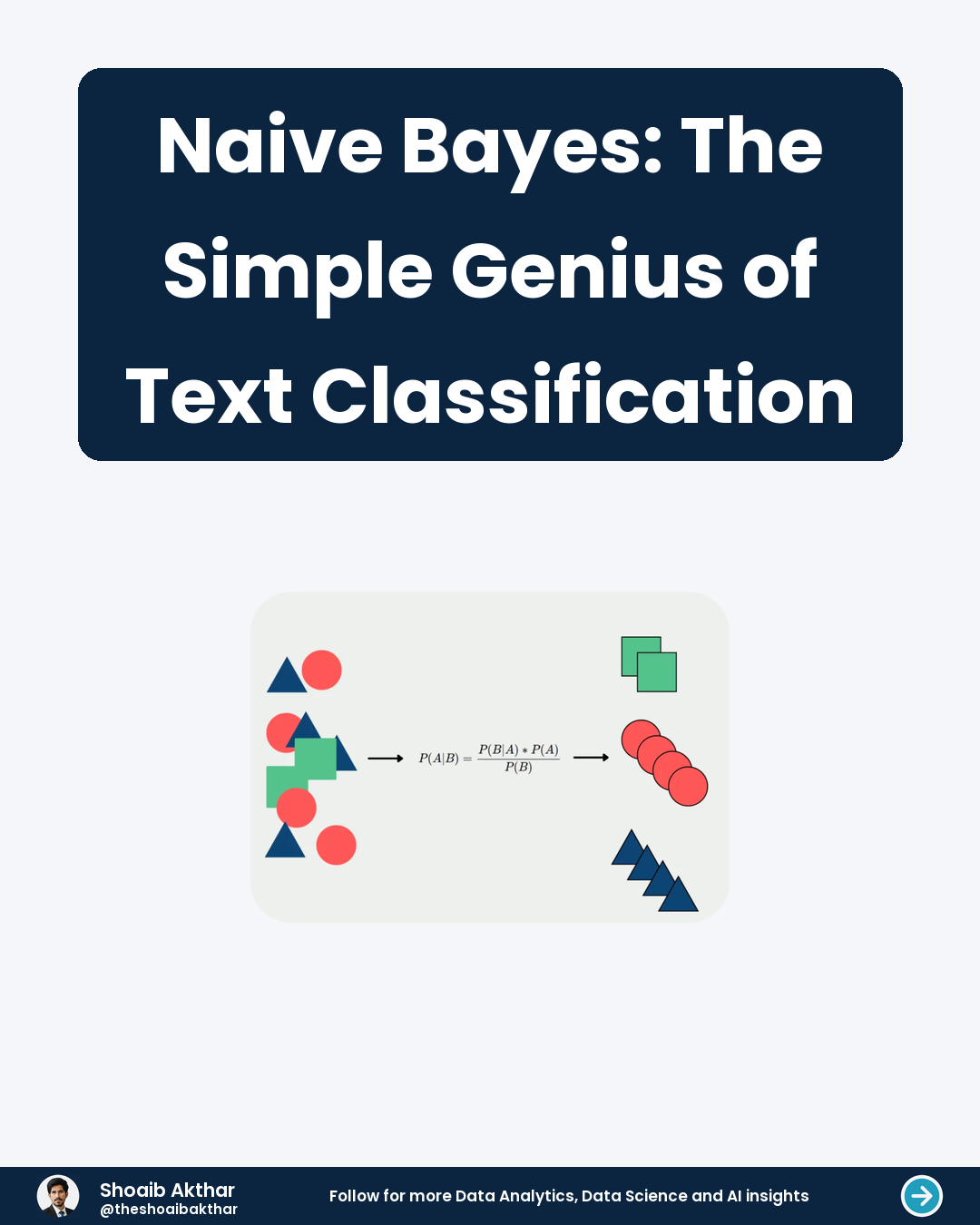
Bayes' Theorem describes the probability of an event based on prior knowledge of conditions related to the event. In our context, we want to find the probability that a document belongs to a certain class, given its features (words).
The formula is written as P(Class | Words) = (P(Words | Class) * P(Class)) / P(Words). We read P(A|B) as "the probability of A given B". For text, we are trying to compute the probability a document is "spam" given the words "win" and "prize".
We calculate this for every possible class and then pick the class with the highest probability. This is known as Maximum A Posteriori (MAP) decision rule.

The problem is that calculating P(Words | Class) for a whole document is complex. The probability of seeing the exact combination of words is very low. This is where the "naive" assumption saves the day.
We naively assume every word in the document appears independently of every other word. This means the position and context of a word do not matter. This allows us to break down the complex probability into a simple product of individual word probabilities.
So, P(Words | Class) becomes P(word1 | Class) * P(word2 | Class) * ... * P(wordN | Class). This makes the math not only possible but also very fast to compute.

The model learns by counting words in a training dataset. It first calculates the prior probability P(Class) for each class. This is just the proportion of documents in the training set that belong to that class.
Then, for each class, it counts how many times each word appears in documents of that class. From these counts, it calculates the likelihood, P(Word | Class), for each word. This is the probability of a word appearing given the document's class.
These calculated probabilities, the priors and the likelihoods, are the entire model. The model is now ready to make predictions on new, unseen documents.

Imagine we are classifying emails as "spam" or "ham". Our training data has 100 emails: 60 ham and 40 spam. The word "win" appears in 2 ham emails and in 20 spam emails.
The prior probabilities are P(ham) = 60/100 = 0.6 and P(spam) = 40/100 = 0.4. The likelihood of "win" given spam is P(win | spam) = 20/40 = 0.5. The likelihood of "win" given ham is P(win | ham) = 2/60 ≈ 0.033.
If a new email contains the word "win", we can see it is much more likely to be spam based on these probabilities.

Its primary power lies in its speed and efficiency. Training and prediction are very fast because the model only involves counting and multiplying probabilities. This makes it ideal for very large datasets where complex models would be too slow.
It often performs surprisingly well, even when the independence assumption is violated. For text classification, it serves as a very strong baseline model. Many more complex algorithms struggle to beat its performance.
It is also less prone to overfitting compared to more complex models, especially with high-dimensional data like text where the number of features (words) is enormous.

A practical problem occurs if a word in a new document never appeared in the training data for a class. Its probability P(word | class) would be zero. Since we multiply all probabilities, this single zero would make the entire product zero.
This is solved using smoothing, most often Laplace smoothing. We add a small value (usually 1) to every word count. This ensures no probability is ever zero. It is a simple but crucial trick that makes the model robust.
For example, with Laplace smoothing, a word that appears 0 times in 40 spam emails would have a probability of (0 + 1) / (40 + total unique words) instead of 0.

Naive Bayes is simple, fast, and highly scalable. Its naive assumption of feature independence is both its greatest weakness and its greatest strength, as it enables efficient computation.
It remains a top choice for text classification tasks like sentiment analysis, spam filtering, and topic categorization. It provides an excellent performance baseline before trying more complex models.
Always remember to use smoothing to handle unseen words. For many real-world applications, its combination of simplicity and power is unbeatable. It is a true workhorse algorithm in machine learning.